Bifract v0.0.3 Release
I’ve been looking forward to putting this one out for a while. Bifract is an open source log management, detection, and collaboration platform built on ClickHouse; if this is your first time hearing about it, the introduction post covers the basics. v0.0.3 is a large release with a lot of work behind it since v0.0.2, and it touches nearly every feature of the project. There are three additions I want to walk through, the provenance graph, models, and an Apache Iceberg archive.
Provenance Graph
A process tree tells you what spawned what. It doesn’t tell you what any of those processes actually did, and on a busy host that’s thousands of events to sort through. The provenance graph, pgr(), is built to close that gap.
Point it at a single process and it rebuilds the spawn tree, then attaches every file write, network connection, DNS query, and injection edge underneath it. Each action gets an anomaly_score from 0 to 1, where 1 is never seen before in your environment and 0 is ubiquitous, and then it prunes.
All of this runs on Sysmon, which is free and something a lot of environments already collect. It isn’t tied to Sysmon, though: anything you normalize into the same categories works just as well, which I put to the test in a follow-up post, running pgr() on EDR telemetry from LimaCharlie.
pgr(start="{GUID}") | pgraph()
pgr() is a source command, so its output is just columns. You can filter, aggregate, sort, and table it like any other query, or pipe it to pgraph() to draw it.
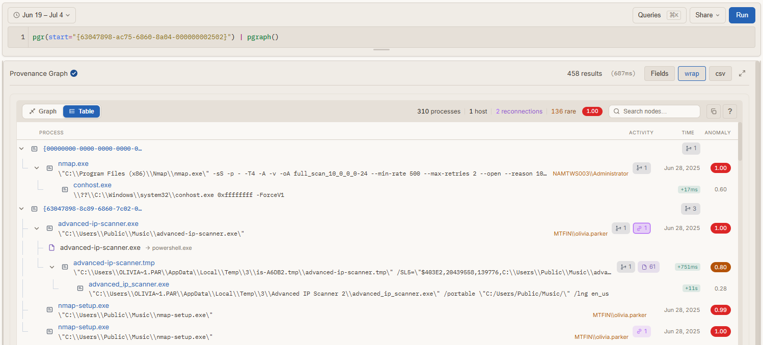
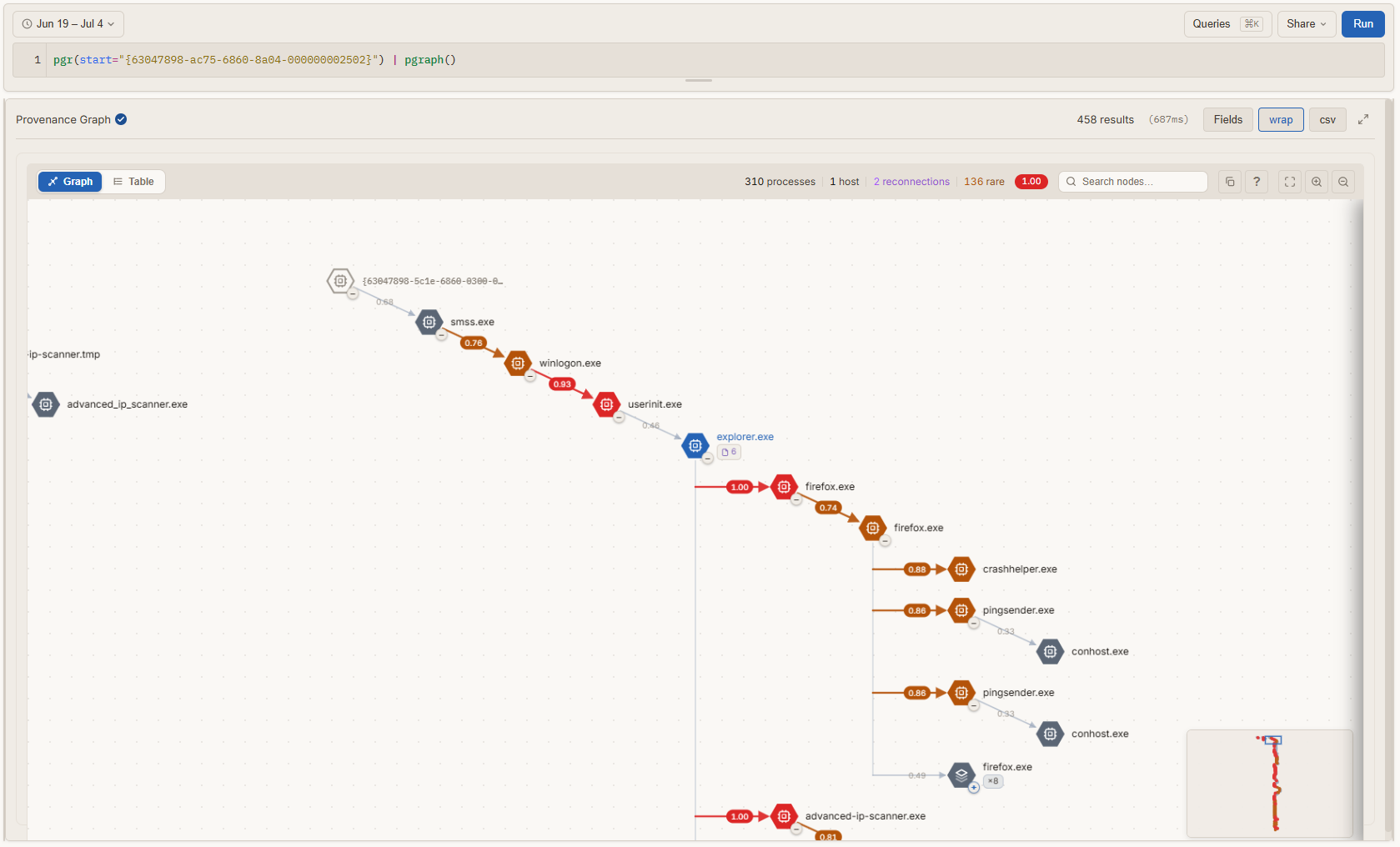
Scoring needs a baseline, so with the feature enabled Bifract maintains two lightweight ones as logs arrive: process lineage (who spawned whom) and behavior frequency (how common each file, IP, and domain is across the fleet). Those baselines abstract before they aggregate. User directories, GUIDs, and long numeric runs collapse to a wildcard, and internal IPs collapse to their /24, so a path under one user’s profile counts as evidence for the same path under another’s. Without that, everything on an endpoint looks rare and the score is useless.
Scores also propagate down the tree, following the NoDoze approach, so a process inherits a decayed share of its parent’s score on top of its own. A chain of mildly unusual steps ends up scoring higher than any single step in it would. This is what living off the land looks like in the data, where every step is a normal binary doing a normal thing and only the sequence is strange, and it’s the case scoring each edge in isolation always misses. Ordinary activity contributes nothing as it propagates, so a long benign chain doesn’t creep upward just for being long.
Attackers also don’t stay inside one process tree. If a process in your tree writes a file and something outside the tree executes it, or two unrelated processes resolve the same rare domain, that’s worth following. Reconnection adds explicit edges through shared files, domains, and resolved IPs so the graph converges on the shared object instead of showing two disconnected halves of the same intrusion.
Performance took most of the work here. Pulling a process’s file, network, and DNS events straight out of the log table means searching for its GUID, and ClickHouse leans on a bloom filter index to skip blocks of rows that can’t contain it. On a busy host that index stops helping, because the GUID turns up in nearly every block and nothing gets skipped. One measurement took 156 seconds and scanned 36 billion rows. Those edges now come from a separate table that Bifract fills as logs arrive, sorted by process GUID, so a lookup jumps straight to a tree’s rows instead of hunting for them. The same read takes 230 milliseconds. It’s pre-aggregated too, so a beaconing process’s thousands of connections to one destination collapse into a single edge.
Because the baselines run on every ingested log, the feature is off by default. An admin turns it on under Settings > Endpoint Behavioral Analytics, and if you don’t use endpoint data you should leave it off. The graph works from whatever categories your normalizer populates: process_creation alone builds the spawn tree, and each additional category adds that layer of activity.
Models
Statistical baselining is not new to security. Rarity scoring, first seen tracking, and volume baselines have been in SIEMs and hunting toolkits for years, and none of the math here is novel. What Models add to Bifract is the ability to build straight from a BQL query without leaving the platform, and to have it maintained continuously against your data.
A model takes a BQL query, captures the matching logs as they arrive, and maintains a compact summary table you can alert on and query against. There are three generic models that work on any log source:
- Rarity, how unusual is a value within its group?
- First seen / Last seen, when was an entity first and last observed?
- Volume Baseline, does an entity’s volume deviate from its own history?
Plus two network models built for Zeek style connection data:
- Beacons
- Long Connections
The network models are heavily inspired by RITA, which has been doing beacon detection on Zeek data for a long time and is worth using on its own. I wanted similar analysis available inline in Bifract, where I can easily cross reference it against other logs, like endpoint data.
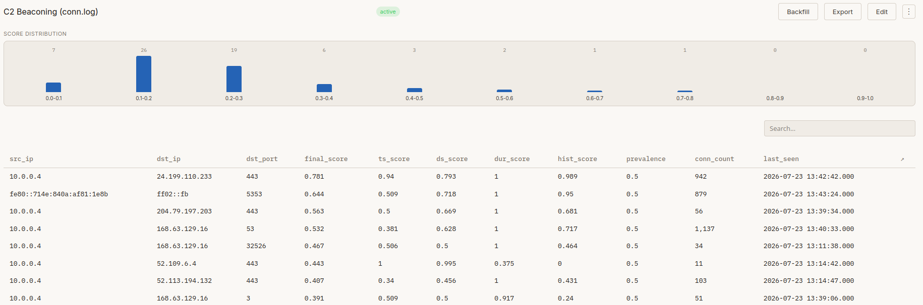
On the backend, models are materialized views feeding aggregating merge tree tables. The work happens once at ingest rather than on every query, which is what makes it viable to keep a baseline running over billions of logs. The tradeoff is that models are forward only, they capture from the moment you create them. If you want history, seed it from the fractal data over a 24h, 7d, 30d, or 90d window.
Every model can carry an alert, new models default to paused, since you don’t yet know what a new baseline looks like in your environment.
Model output is also queryable from BQL with model_lookup(), which joins a model’s results back into a normal search. The model and the search don’t have to share a log source, which is the cross referencing I was after:
event_id=3
| model_lookup(model="zeek_beacons", key=[src_ip, dst_ip, dst_port])
| beacon_score > 0.5
| table(timestamp,image,dst_ip,dst_port,beacon_score,prevalence)
The model here is built on Zeek conn.log, but the search runs over Sysmon event ID 3, network connections. Zeek can see the timing well enough to score a beacon, but has no idea which process opened the connection. Sysmon knows the process and nothing about the pattern. Joining on source, destination, and port gives you a scored beacon with a process image attached to it.
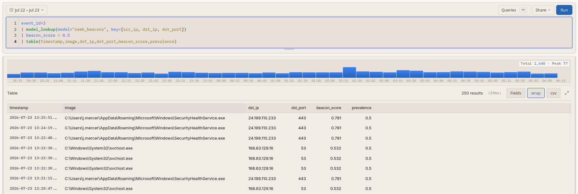
In this case that’s SecurityHealthService.exe beaconing to 24.199.110[.]233 on 443. That’s a real Windows binary name, but it’s running out of AppData\Roaming instead of System32.
Each model type exposes its own output columns, so a rarity lookup gives you percent, confidence, and model_count, while a first/last seen lookup gives you first_seen, last_seen, and is_new. Models export to YAML, so they can live in version control and move between fractals and deployments.
Apache Iceberg
In this release I’ve added Apache Iceberg as a way to store data longer than what you keep directly in ClickHouse, as well as a method of recovering from critical failures.
With it enabled, every ingested log is written to object storage (e.g., S3-compatible, Azure Blob) as Parquet with Iceberg metadata, independent of ClickHouse. ClickHouse becomes a bounded hot window governed by each fractal’s retention, and the archive holds the full history.
Parquet and Iceberg are open formats, which means any Iceberg-compatible reader can query the archive directly, even with Bifract gone. Here’s DuckDB reading one, no export step and nothing from Bifract in the loop:
INSTALL iceberg; LOAD iceberg;

CREATE SECRET archive (TYPE s3, KEY_ID '...', SECRET '...');

SELECT json_extract_string(norm_log, '$.event_id') AS event_id, count(*) AS n
FROM iceberg_scan('s3://your-bucket/bifract.db/f_<fractal-id>')
GROUP BY 1 ORDER BY n DESC;
Frequently queried fields are promoted to typed columns, the full normalized event is JSON in norm_log, and the original is in raw_log.
PyIceberg works too, and since it can attach to the same catalog Bifract writes through, it enumerates every fractal’s table rather than needing to be pointed at one.
Recall
Recall queries the Iceberg archive in place. It looks like a normal search, but every run is a server-side job that reads Parquet directly from object storage. The job runs server side, so navigating away or refreshing never cancels, and you can return to review the results.
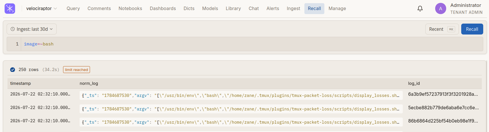
In a critical DR scenario you can restore recent logs from the archive back into ClickHouse, enough to get search, alerting, and dashboards working again. If you’re reaching for a multi-month restore to answer an investigative question, Recall is probably the right tool instead.
Benchmark
The first question anyone asks is whether it handles their volume, so I ran a sustained 24 hour load test on DigitalOcean Kubernetes.
This is the upper end of what I’ve tested, not what it takes to get started. Bifract installs on a single Linux host with one command, and a single node covers most deployments; the cluster below is what the same software looks like when you scale it out.
Three ClickHouse shards at 32 vCPU and 64GB each, plus two nodes for the app and ingest tiers. The load generator ships in the repo as bifract-loadgen. It emits Sysmon shaped events built to resemble a real fleet rather than random noise: a few domains and destination IPs show up constantly while most are rare, hashes stay fixed per binary instead of changing every event, and each process reuses one GUID across its file, network, and DNS activity so the provenance edges are real.
Over the full 24 hours it sustained:
- 9,798 events per second, 5.95 MB/s, 502 GB delivered
- p50 of 125ms and p95 of 230ms, measured while ingesting
- 382 rejections out of 1.69 million requests, and no other errors
- 65% compression on the log table, though that number moves a lot with log shape; on other data I’ve had it sit closer to 75%
That’s with endpoint behavioral analytics running and 932 Sigma rules evaluating against the same cluster. Alert evaluation dragged ingest down on an earlier deployment, so I’d already moved it onto a teed copy: a separate table holding only a few hours of data that alerting evaluates against instead of the full log store. Neither the analytics nor the rules showed up in the ingest numbers here. Keeping them on that small window rather than the whole history is what took the load off ClickHouse.
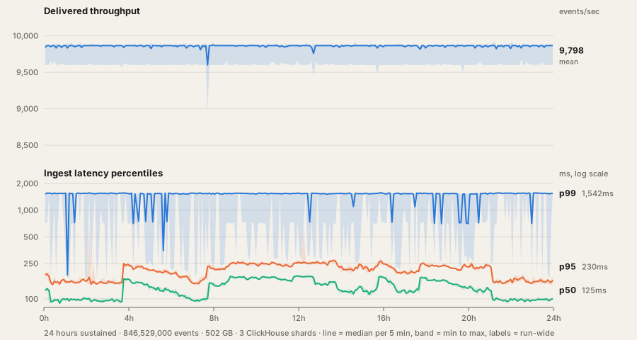
p50 is the median request and p95 is the slowest one in twenty, so together they describe both what a normal request costs and how bad the slow ones get. The second number is the one I care about, because a system can sit at a healthy median while a steady slice of requests stalls for seconds, and averages hide that completely.
The real ceiling turned out to be the managed load balancer in front of the cluster, not the cluster itself. At its default size, p50 sat at a healthy 45ms while p99, the slowest request in a hundred, stalled at 19 seconds. Resizing it brought p99 down to the level you see above, and p50 rose only because the cluster was finally taking full throughput. Nothing inside the cluster ever looked saturated, which is exactly why the slowest requests are the ones to watch.

Query Language
BQL got three new operators for multi-term matching:
image=~powershell,pwsh,cmd
image=^mimikatz,impacket
image=$exe,dll,bat
=~ is contains-any, =^ is starts-with-any, and =$ is ends-with-any, all case insensitive against a comma separated list. They’re faster than the equivalent regular expression because they compile down to ClickHouse’s multi-search string functions and pick up additional speed from available text indexes. Most of the regex I was writing was really just “does this field contain one of these strings”, which is served much better by these new operators. Regular expressions of course remain available for when you need them.
case statements let you branch a query and run different pipe commands down each branch. Here every event is tagged with whether it was enriched, then charted over time in a single pass:
artifact = Custom.Linux.Events.EBPF
| case {
  tracker_hit=true | process_enriched:=true;
  * | process_enriched:=false;
}
| timechart(span=15m,function=percent(process_enriched,parent_enriched))
There’s also logSize(), which returns the byte size of a log at query time. It works retroactively over all your data with no extra storage, which makes it a quick way to find out what’s driving your ingest volume:
* | logSize() | groupby(computer_name, function=sum(_size))
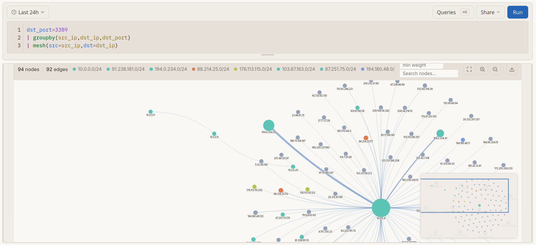
mesh() draws a graph from grouped connection data, one node per host and an edge for each pair that talked. Here it maps every RDP connection, and a host reaching out to a fan of external addresses on 3389 stands out at a glance:
dst_port=3389
| groupby(src_ip,dst_ip,dst_port)
| mesh(src=src_ip,dst=dst_ip)
Everything Else
The rest of the release is full of redesign and performance work:
- Streaming results. Queries stream results back in windows with a cancel button, and the histogram and results table load asynchronously, so a broad query over a long window is usable before it finishes.
- Query performance. Token prefiltering, PREWHERE usage, default bloom filter and set indexes on built-in fields, and a much faster log details pane.
- Schema tab. An admin-only page for promoting frequently filtered attributes to indexed schema fields, with bloom filter or set indexes depending on cardinality, plus YAML import and export.
- Shared dashboard links. Publish a dashboard to a link that renders server side.
- MCP server. The MCP server gained tools for the provenance graph, field discovery, behavioral models, and dashboards, so an agent can seed
pgr()on a process and read the scored tree back without leaving the terminal. Client certificates and private CAs are supported for instances behind mTLS. - Ingestion. Ingest runs in its own containers separate from the app, with per-fractal partitioning, better shard balancing on Kubernetes, and dropped log tracking.
Conclusion
The provenance graph cuts endpoint noise down to what’s worth looking at, models give you baselines alongside your rules, and the Iceberg archive means your data outlives the database serving it. The archive is the newest and least proven of the three, and it’s the piece I expect to change most in the next few releases.
Check out the docs to get started, browse the source on GitHub, or star the repo if the project interests you. Issues and contributions are always welcome.